Dynamics (sbpy.dynamics)

sbpy has the capability to describe dynamical states (position and velocity vectors), and to integrate test particle orbits. These are primarily intended to support the generation of Dust syndynes and synchrones.

Dynamical state

State objects encapsulate the position and velocity of an object at a given time. Create a State for a comet at \(x=2\) au, moving along the y-axis at a speed of 30 km/s:

>>> from astropy.time import Time
>>> import astropy.units as u
>>> from sbpy.dynamics import State
>>>
>>> r = [2, 0, 0] * u.au
>>> v = [0, 30, 0] * u.km / u.s
>>> t = Time("2023-12-08")
>>> comet = State(r, v, t)

State objects may also represent an array of objects:

>>> r = ([2, 0, 0], [0, 2, 0]) * u.au
>>> v = ([0, 30, 0], [30, 0, 0]) * u.km / u.s
>>> t = Time(["2023-12-08", "2023-12-09"])
>>> comets = State(r, v, t)
>>> len(comets)
2

The r, v, and t attributes hold the position, velocity, and time for the object(s). The first index iterates over the object, the second iterates over the x-, y-, and z-axes.

>>> comets.r.shape
(2, 3)
>>> comets.r[0]
<Quantity [2., 0., 0.] AU>

Or, index the State object itself:

>>> comets[0].r  # equivalent to comets.r[0]
<Quantity [2., 0., 0.] AU>

Convert to/from Ephem and SkyCoord

State objects may be initialized from ephemeris objects (Ephem), provided they contain time, and 3D position and velocity:

>>> from sbpy.data import Ephem
>>> eph = Ephem.from_horizons("9P",
...                           epochs=Time("2005-07-04"),
...                           id_type="designation",
...                           closest_apparition=True)
>>> tempel1 = State.from_ephem(eph)

And State may be converted to an Ephem object:

>>> eph = tempel1.to_ephem()

astropy’s SkyCoord objects may also be used, assuming the time and 3D vectors are fully defined:

>>> from astropy.coordinates import SkyCoord
>>> coords = SkyCoord(ra="01:02:03h",
...                   dec="+04:05:06d",
...                   pm_ra_cosdec=100 * u.arcsec / u.hr,
...                   pm_dec=-10 * u.arcsec / u.hr,
...                   distance=1 * u.au,
...                   radial_velocity=15 * u.km / u.s,
...                   obstime=Time("2024-01-19"))
>>> state = State.from_skycoord(coords)

And back to a SkyCoord object:

>>> state.to_skycoord()
<SkyCoord (ICRS): (x, y, z) in AU
    (0.96112414, 0.26676914, 0.07123631)
 (v_x, v_y, v_z) in km / s
    (9.16701924, 23.45244422, -0.94097856)>

Reference frames

Coordinate reference frames can be specified with the frame keyword argument during initialization. Most of astropy reference frames are supported (see astropy’s Built-in Frame Classes):

Note

When working with heliocentric ecliptic coordinates from JPL Horizons or NAIF SPICE, you may want to use the HeliocentricEclipticIAU76 reference frame.

>>> r = [2, 0, 0] * u.au
>>> v = [0, 30, 0] * u.km / u.s
>>> t = Time("2023-12-08")
>>> state = State(r, v, t, frame="heliocentriceclipticiau76")
>>> state
<State (<HeliocentricEclipticIAU76 Frame (obstime=2023-12-08 00:00:00.000)>):
 r
  [2. 0. 0.] AU
 v
  [ 0. 30.  0.] km / s
 t
  2023-12-08 00:00:00.000>

Use transform_to() to transform between reference frames:

>>> new_state = state.transform_to("icrs")
>>> new_state
 <State (<ICRS Frame>):
  r
   [ 1.99191790e+00 -2.59236051e-03 -8.93633307e-04] AU
  v
   [8.11760173e-03 2.75129298e+01 1.19282350e+01] km / s
  t
   2023-12-08 00:00:00.000>

State lengths, subtraction, and observations

A few mathematical operations are possible. Get the magnitude of the heliocentric distance and velocity with abs:

>>> print(abs(comet))
(<Quantity 2. AU>, <Quantity 30. km / s>)

Get the Earth-comet state vector by subtraction:

>>> earth = State([0, 1, 0] * u.km, [30, 0, 0] * u.km / u.s, comet.t)
>>> print(comet - earth)
<State (<ArbitraryFrame Frame>):
 r
  [ 2.00000000e+00 -6.68458712e-09  0.00000000e+00] AU
 v
  [-30.  30.   0.] km / s
 t
  2023-12-08 00:00:00.000>

Or, get the sky coordinates of the comet as seen from the Earth:

>>> earth.observe(comet)
<SkyCoord (ArbitraryFrame): (lon, lat, distance) in (deg, deg, AU)
    (359.99999981, 0., 2.)
 (pm_lon, pm_lat, radial_velocity) in (mas / yr, mas / yr, km / s)
    (6.52671946e+08, 0., -30.0000001)>

The result, a SkyCoord object, is expressed in the reference frame of the observer.

Fetching states from Horizons

Ephem.from_horizons returns equatorial coordinates in the ICRF reference frame, which has its origin at the Solar System barycenter. For State to correctly convert the ephemeris object to vectors, we need to set the Horizons observer to the Solar System barycenter ("@ssb"). However, dynamical integrations are done in a heliocentric reference frame, so we transform the result to "heliocentriceclipticiau76":

>>> eph = Ephem.from_horizons(
...     "48P",
...     id_type="designation",
...     closest_apparition=True,
...     epochs=Time("2004-10-13T21:08:23.894"),
...     location="@ssb",
... )
>>> comet = State.from_ephem(eph, frame="icrs")
>>> comet = comet.transform_to("heliocentriceclipticiau76")

Dynamical integrators

A state object may be propagated to a new time using a dynamical integrator. Three integrators are defined. Use FreeExpansion for motion in free space, SolarGravity for orbits around the Sun, and SolarGravityAndRadiationPressure for orbits around the Sun considering radiation pressure.

>>> from sbpy.dynamics import SolarGravity
>>> state = State([1, 0, 0] * u.au, [0, 30, 0] * u.km / u.s, 0 * u.s)
>>> integrator = SolarGravity()
>>> t_final = 1 * u.year
>>> integrator.solve(state, t_final)
<State (<ArbitraryFrame Frame>):
 r
  [ 1.48146925e+08 -2.09358771e+07  0.00000000e+00] km
 v
  [ 4.137801   29.70907176  0.        ] km / s
 t
  1.0 yr>

Other integrators may be defined. Use the above classes as templates or as base classes. For example, to simulate orbits around the Earth, update the _GM private attribute from SolarGravity:

>>> class EarthGravity(SolarGravity):
...     _GM = 3.9860043543609598e5  # km3/s2

Dust syndynes and synchrones

Syndynes are lines in space connecting particles that are experiencing the same forces. A syndyne is parameterized by \(\beta\), the ratio of the force from solar radiation to the force from solar gravity, \(F_r / F_g\), and age (or time of release). Thus, all particles in a syndyne have a constant \(\beta\) but variable age. Similarly, synchrones are lines of constant particle age, but variable \(\beta\).

Start with a SynGenerator

sbpy has the sbpy.dynamics.syndynes.SynGenerator class to assist the user in the generation of syndynes, synchrones, and points along a source object’s orbit. Use the SynGenerator’s syndynes(), synchrones(), and source_orbit() methods to produce Syndynes, Synchrones, and SourceOrbit objects, described in further detail below.

Setting up a SynGenerator instance requires a dust source, and dust \(\beta\) values and ages from which to generate the syndynes/synchrones.

First, define the dust source, a comet at 2 au from the Sun:

>>> from astropy.time import Time
>>> import astropy.units as u
>>> from sbpy.dynamics import State
>>>
>>> r = [2, 0, 0] * u.au
>>> v = [0, 30, 0] * u.km / u.s
>>> t = Time("2023-12-08")
>>> comet = State(r, v, t)

Next, initialize the syn-generator object. Here, we request dust with \(\beta\) values from 0 to 1, generated over a 100-day period:

>>> import numpy as np
>>> from sbpy.dynamics import SynGenerator
>>>
>>> betas = [1, 0.1, 0.01, 0]
>>> ages = np.linspace(0, 100, 26) * u.day
>>> dust = SynGenerator(comet, betas, ages)
>>> dust
<SynGenerator:
betas
   [1.   0.1  0.01 0.  ]
ages
   [  0.   4.   8.  12.  16.  20.  24.  28.  32.  36.  40.  44.  48.  52.
 56.  60.  64.  68.  72.  76.  80.  84.  88.  92.  96. 100.] d>

The computed particle positions are saved in the particles attribute. For our example, the 4 \(\beta\)-values and the 26 ages produce 104 particles:

>>> print(len(dust.particles))
104

Syndynes

Zero-ejection velocity syndynes are generated with the SynGenerator class, and this example uses the generator above. Get the syndynes with the syndynes() method, which returns Syndynes a list-like collection of Syndyne objects (note the use of plural and singular forms).

>>> syndynes = dust.syndynes()
>>> syndynes
<Syndynes: betas=[1.   0.1  0.01 0.  ]>
>>> syndynes[0]
<Syndyne (<ArbitraryFrame Frame>):
 r
  [[ 2.99195741e+08  0.00000000e+00  0.00000000e+00]
 [ 2.99284224e+08 -2.04410384e+03  0.00000000e+00]
 [ 2.99549029e+08 -1.63231106e+04  0.00000000e+00]
 [ 2.99988249e+08 -5.49241301e+04  0.00000000e+00]
 [ 3.00598735e+08 -1.29642418e+05  0.00000000e+00]
...

Syndyne objects are specialized State objects. For example, we can compute the linear distance from the comet to farthest particle in each syndyne:

>>> for syndyne in dust.syndynes():
...     r, v = abs(syndyne - comet)
...     print(syndyne.beta, "{:.3f}".format(r.max().to("au")), sep=", ")
1.0, 0.309 AU
0.1, 0.032 AU
0.01, 0.003 AU
0.0, 0.000 AU

Individual syndynes may also be retrieved directly from the SynGenerator object using the syndyne() method and a syndyne index. The index for the syndyne matches the index of the betas array, i.e., to get the \(\beta=0.1\) syndyne from our example:

>>> print(dust.betas)
[1.   0.1  0.01 0.  ]
>>> syndyne = dust.syndyne(1)
>>> print(syndyne.beta)
0.1

Synchrones

Synchrones are also simulated with the SynGenerator class, but instead retrieved with the synchrone() and synchrones() methods, which return Synchrone objects, or collections thereof:

>>> synchrone = dust.synchrone(24)
>>> r, v = abs(synchrone)
>>> print(synchrone.age, "{:.3g}".format(r.max().to("au")), sep=", ")
96.0 d, 2.26 AU

To support generating synchrones at specific times, the at_epochs() method may be used to initialize a SynGenerator:

>>> dates = Time(["2023-10-01", "2023-11-01", "2023-12-01"])
>>> dust = SynGenerator.at_epochs(comet, betas, dates)
>>> synchrone = dust.synchrone(0)
>>> synchrone.epoch
<Time object: scale='utc' format='iso' value=2023-10-01 00:00:00.000>

Source object’s orbit

The SynGenerator can also generate points along the source object’s oribit. Calculating the positions of the projected orbit of the source object may be helpful for comparison to syndynes, or a comet’s dust trail. They are calculated with the source_orbit() method. To produce 3 points at -2, 0, and +2 days from the object’s current position:

>>> dt = np.linspace(-2, 2, 3) * u.d
>>> orbit = dust.source_orbit(dt)

This method produced a SourceOrbit object that is functionally the same as the Syndynes and Synchrones objects above:

>>> type(orbit)
<class 'sbpy.dynamics.syndynes.SourceOrbit'>
>>> orbit.ages
<Quantity [ 2., -0., -2.] d>
>>> np.linalg.norm(orbit[0].r - orbit[1].r)
<Quantity 5183919.42549707 km>

Adding ejection velocity

An ejection velocity can be added to the dust particles. This is not implemented in sbpy, but is possible by sub-classing SynGenerator and overriding the initialize_states method. In the following example we add 10 m/s to the z-component of the velocity:

>>> class AlternativeSynGenerator(SynGenerator):
...     def initialize_states(self):
...         super().initialize_states()
...         delta_v = State([0, 0, 0] * u.km, [0, 0, 0.01] * u.km / u.s, 0)
...         self.initial_states = self.initial_states + delta_v
>>>
>>> dust_with_delta_v = AlternativeSynGenerator.at_epochs(comet, betas, dates)
>>> dust_with_delta_v.initial_states - dust.initial_states
 <State (<ArbitraryFrame Frame>):
 r
  [[0. 0. 0.]
 [0. 0. 0.]
 [0. 0. 0.]] km
 v
  [[0.   0.   0.01]
 [0.   0.   0.01]
 [0.   0.   0.01]] km / s
 t
  ['2023-10-01 00:00:00.000' '2023-11-01 00:00:00.000'
 '2023-12-01 00:00:00.000']>

Projecting onto the sky

Syndynes and synchrones may be projected onto the sky as seen by a telescope. This requires an observer. For precision work, the SynGenerator source object’s State should be defined in a heliocentric reference frame. Typically, the observer will observe in an equatorial reference frame, but your needs may vary. Here, we generate syndynes in the HeliocentricEclipticIAU76 coordinate frame, which is the same J2000 heliocentric ecliptic coordinate frame that JPL Horizons and the NAIF SPICE toolkit use. We then observe the results in the ICRS reference frame:

>>> r = [2, 0, 0] * u.au
>>> v = [0, 30, 0] * u.km / u.s
>>> t = Time("2023-12-08")
>>> comet = State(r, v, t, frame="heliocentriceclipticiau76")
>>> observer = State(
...     r=[0, 2, 2] * u.au,
...     v=[0, 0, 0] * u.km / u.s,
...     t=comet.t,
...     frame="icrs",
... )
>>> dust = SynGenerator(comet, betas, ages, observer=observer)

With the observer and coordinate frames defined, the generated syndynes and synchrones will have a coords attribute, which is an astropy.coordinates.SkyCoord object representing the sky positions of the test particles. Here, we print a sample of the coordinates:

>>> syndyne = dust.syndyne(0)
>>> print("\n".join(syndyne.coords[::5].to_string("hmsdms", precision=0)))
20h59m23s -35d18m48s
21h00m08s -35d12m50s
21h01m53s -34d55m44s
21h03m49s -34d30m22s
21h05m19s -34d00m41s
21h05m59s -33d30m26s

Using other dynamical models

sbpy’s built-in models solve the equations of motion for dust grains given two-body dynamics. Users may provide their own models in order to, e.g., improve code performance, add planetary perturbations, model grain fragmentation, etc.. Use the SolarGravityAndRadiationPressure class as a template.

In this example, we compute the syndynes of a comet orbiting β Pic (1.8 solar masses) by sub-classing SolarGravityAndRadiationPressure and updating \(GM\), the mass of the star times the gravitational constant:

>>> import astropy.constants as const
>>> from sbpy.dynamics import SolarGravityAndRadiationPressure
>>>
>>> class BetaPicGravityAndRadiationPressure(SolarGravityAndRadiationPressure):
...     _GM = 1.8 * SolarGravityAndRadiationPressure._GM
>>>
>>> solver = BetaPicGravityAndRadiationPressure()
>>> betapic_dust = SynGenerator(comet, [1, 0], [0, 100] * u.d, solver=solver)

Plotting syndynes, synchrones, and orbits

Generally, we are interested in visualizing the syndynes and synchrones for an observer. Syndynes, Synchrones, and SourceOrbit objects have plot() methods to assist with this. They can plot the coordinates relative to the comet with a simple tangent plane projection, or projected onto the image plane with an astropy.wcs.WCS object.

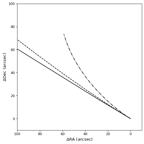
Here is an example that plots the syndynes and synchrones from above as offsets from the comet’s coordinates:

>>> import matplotlib.pyplot as plt
>>>
>>> fig, ax = plt.subplots()
>>>
>>> # plot all but the last (beta=0) syndyne
>>> syndynes = dust.syndynes()
>>> syndynes[:-1].plot(ax)
>>>
>>> # plot every 5th synchrone
>>> synchrones = dust.synchrones()
>>> synchrones[4::5].plot(ax, ls="--")
>>>
>>> # plot the orbit
>>> dt = np.linspace(-2, 2) * u.d
>>> orbit = dust.source_orbit(dt)
>>> orbit.plot(ax, color="k", ls=":", label="Orbit")
>>>
>>> ax.invert_xaxis()
>>> ax.set(
...     xlim=[100, -10],
...     ylim=[-10, 100],
...     xlabel="$\\Delta$RA (arcsec)",
...     ylabel="$\\Delta$Dec (arcsec)",
... )
>>> ax.legend()
>>> fig.tight_layout()

(png, svg, pdf)

For more complex plot logic, e.g., specific line colors and styles, use the plot methods of the individual syndynes/synchrones:

>>> ls = ["-", "--", "-."]
>>> syndynes = dust.syndynes()
>>> for i in range(3):
...     syndynes[i].plot(ax, color="k", ls=ls[i])

(Source code, png, svg, pdf)

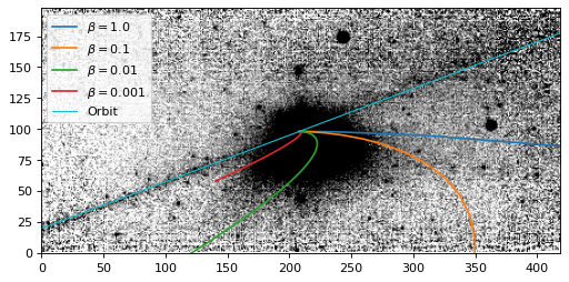
The following complete example compares syndynes to a Spitzer Space Telescope image of comet 48P/Johnson (Reach et al. 2007). The FITS world coordinate system is used to account for the image orientation and scale. To precisely align the syndynes with the comet nucleus, we update the world coordinate system to use our calculated comet coordinates.

Note

The sbpy testing suite shows that arcsecond-level accuracy is possible, but this is generally not enough for direct comparison to typical images of comets, which need sub-arcsecond alignment. The accuracy of the coordinates object depends on the the comet and observer states, but also on whether or not light travel time is accounted for, and the accuracy of the orbit integrator. In the following example, the world coordinate system is edited to manually align the image and syndynes.

>>> from astropy.io import fits
>>> from astropy.wcs import WCS
>>>
>>> image, header = fits.getdata("https://sbpy.org/data/48p-spitzer-reach07.fits", header=True)
>>> obstime = Time(header["DATE_OBS"])
>>>
>>> # get the comet state
>>> eph = Ephem.from_horizons(
...     "48P",
...     id_type="designation",
...     closest_apparition=True,
...     epochs=obstime,
...     location="@ssb",
... )
>>> comet = State.from_ephem(eph, frame="icrs")
>>> comet = comet.transform_to("heliocentriceclipticiau76")
>>>
>>> # get the Spitzer Space Telescope state
>>> eph = Ephem.from_horizons("-79", id_type=None, epochs=obstime, location="@ssb")
>>> observer = State.from_ephem(eph, frame="icrs")
>>>
>>> # set up the world coordinate system object and update the origin to align with
>>> # the calculated position of the comet
>>> wcs = WCS(header)
>>> coords0 = observer.observe(comet)[0].unmasked
>>> wcs.wcs.crval = coords0.ra.deg, coords0.dec.deg
>>> wcs.wcs.crpix = 209, 99
>>>
>>> # generate the syndynes
>>> betas = [1, 0.1, 0.01, 0.001]
>>> ages = np.linspace(0, 365, 51) * u.day
>>> dust = SynGenerator(comet[0], betas, ages, observer=observer[0])
>>>
>>> # plot the image and syndynes
>>> fig, ax = plt.subplots(num=1, clear=True, figsize=(6.5, 3.25))
>>>
>>> ax.imshow(image, origin="lower", vmin=49.1, vmax=49.5, cmap="gray_r")  # docte
>>>
>>> # save xlim and ylim for later
>>> xlim = ax.get_xlim()
>>> ylim = ax.get_ylim()
>>>
>>> # plot syndynes
>>> syndynes = dust.syndynes()
>>> syndynes.plot(ax, wcs=wcs)
>>>
>>> # plot the orbit
>>> dt = np.linspace(-1, 1) * u.d
>>> orbit = dust.source_orbit(dt)
>>> orbit.plot(ax, wcs=wcs, color="tab:cyan", lw=1, label="Orbit")
>>>
>>> ax.set(xlim=xlim, ylim=ylim)
>>> ax.legend()

(Source code, png, svg, pdf)

Reference/API

sbpy.dynamics.state Module

Classes

ArbitraryFrame(*args[, copy, ...])	Coordinate frame with arbitrary space and time references.
StateBase(r, v, t[, frame])	Abstract base class for dynamical state.
State(r, v, t[, frame])	Dynamical state.
SolverFailed	DynamicalModel solver failed.

Class Inheritance Diagram

sbpy.dynamics.models Module

Classes

DynamicalModel(**kwargs)	Super-class for dynamical models.
FreeExpansion(**kwargs)	Equation of motion solver for particle motion in free space.
SolarGravity(**kwargs)	Equation of motion solver for a particle orbiting the Sun.
SolarGravityAndRadiationPressure(**kwargs)	Equation of motion solver for a particle orbiting the Sun, including radiation force.
SolverFailed	DynamicalModel solver failed.

Class Inheritance Diagram

sbpy.dynamics.syndynes Module

Classes

SourceOrbit(source, dt, r, v, t[, observer])	Collection of states that make up an orbit.
SynGenerator(source, betas, ages[, ...])	Syndyne / synchrone generator for cometary dust.
SynStates(source, betas, ages, r, v, t, initial)	Abstract base class for particle states that make up a syndyne or synchrone.
SynCollection(items)	Immutable collection of syndynes or synchrones.
Syndyne(source, beta, ages, r, v, t, initial)	Collection of particle states that make up a syndyne.
Syndynes(items)	Collection of syndynes.
Synchrone(source, betas, age, r, v, t, initial)	Collection of particle states that make up a synchrone.
Synchrones(items)	Collection of synchrones.

Class Inheritance Diagram